Real-time ad performance analysis
RisingWave makes it possible to do real-time ad performance analysis in a low code manner.
Overview
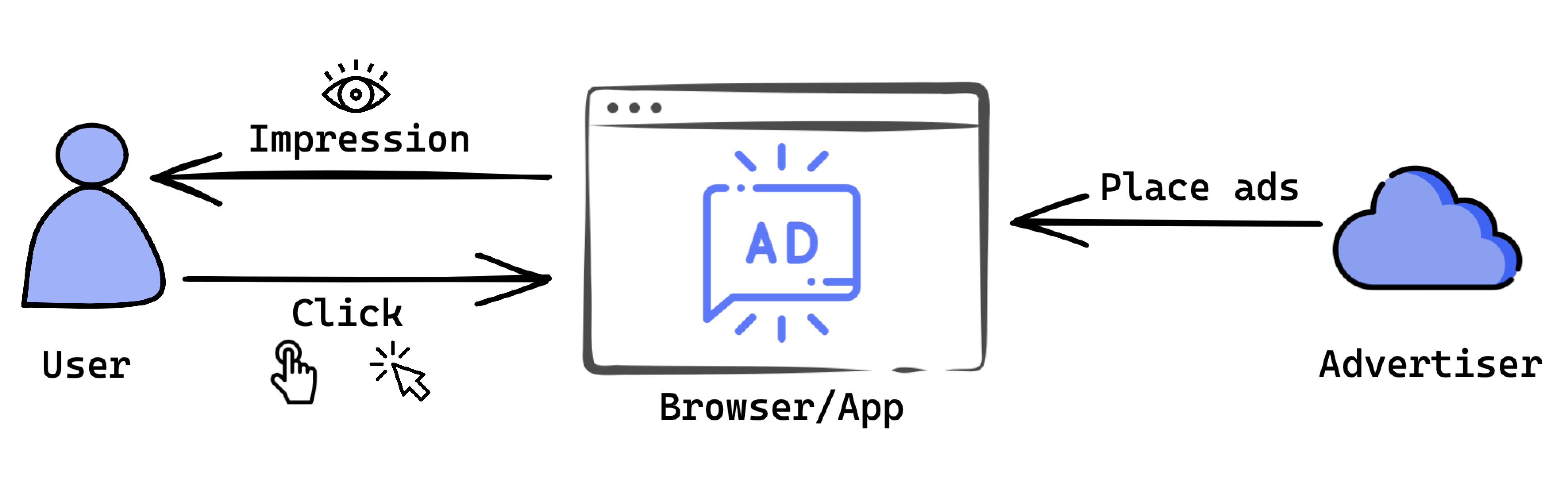
Ad platforms and advertisers alike want to measure the performance of their ads. They implement events that will be triggered and sent back to their servers upon certain user interactions (viewing or clicking an ad, installing an app, or making a purchase) on websites or mobile applications. Based on these events, they define various metrics to analyze ad performance from different angles.
Click-through rate (CTR) is one of the key metrics used in digital advertising to gauge the effectiveness of ads. It is calculated as the number of clicks divided by the number of impressions. Impressions are the number of times a digital ad displays on someone's screen in an app or on a website. A high CTR means that users find the ads displayed to them useful and relevant.
In this tutorial, you will learn how to get real-time click-through rates from ad impressions and click events with RisingWave. We have set up a demo cluster specifically for this tutorial so that you can try it out with ease.
Prerequisites
- Ensure you have Docker and Docker Compose installed in your environment. Note that Docker Compose is included in Docker Desktop for Windows and macOS. If you use Docker Desktop, ensure that it is running before launching the demo cluster.
- Ensure that the PostgreSQL interactive terminal,
psql, is installed in your environment. For detailed instructions, see Download PostgreSQL.
Step 1: Launch the demo cluster
In the demo cluster, we packaged RisingWave and a workload generator. The workload generator will start to generate random traffic and feed them into Kafka as soon as the cluster is started.
First, clone the risingwave repository to the environment.
git clone https://github.com/risingwavelabs/risingwave.git
Now navigate to the integration_tests/ad-ctr directory and start the demo cluster from the docker compose file.
cd risingwave/integration_tests/ad-ctr
docker compose up -d
The default command-line syntax in Compose V2 starts with docker compose. See details in the Docker docs.
If you're using Compose V1, use docker-compose instead.
Necessary RisingWave components, including compute node, metadata node, and MinIO, will be started. The workload generator will start to generate random data and feed them into Kafka topics. In this demo cluster, data of materialized views will be stored in the MinIO instance.
Step 2: Connect RisingWave to data streams
Now let's connect to RisingWave so that we can manage data streams and perform data analysis.
psql -h localhost -p 4566 -d dev -U root
We'll treat ad impressions and ad click events as separate streams and use simplified schemas so that you can get the gist easily.
Below is the schema of ad impression events. In this schema, impression_timestamp is the date and time when an ad is presented to a viewer, and bid_id is the identifier of a bid request or activity for an online ad. When we calculate click-through rates, we must make sure that the impressions and the clicks are for the same bid request / activity. Otherwise, the results will be meaningless.
{
  "bid_id": 2439384144522347,
  "ad_id": 5,
  "impression_timestamp": "2022-05-23T14:11:04Z"
}
The schema of ad click events is like this:
{
  "bid_id": 2439384144522347,
  "click_timestamp": "2022-05-23T14:12:56Z"
}
For the same bid ID, impression_timestamp should always be smaller (earlier) than click_timestamp.
Now that we already set up these two data streams in Kafka (in JSON) using the demo cluster, we can connect to these two streams with the following SQL statements.
CREATE SOURCE ad_impression (
    bid_id BIGINT,
    ad_id BIGINT,
    impression_timestamp TIMESTAMP WITH TIME ZONE
) WITH (
    connector = 'kafka',
    topic = 'ad_impression',
    properties.bootstrap.server = 'message_queue:29092',
    scan.startup.mode = 'earliest'
) FORMAT PLAIN ENCODE JSON;
CREATE SOURCE ad_click (
    bid_id BIGINT,
    click_timestamp TIMESTAMP WITH TIME ZONE
) WITH (
    connector = 'kafka',
    topic = 'ad_click',
    properties.bootstrap.server = 'message_queue:29092',
    scan.startup.mode = 'earliest'
) FORMAT PLAIN ENCODE JSON;
scan.startup.mode = 'earliest' means the source will start streaming from the earliest entry in Kafka. Internally, RisingWave will record the consumed offset in the persistent state so that during a failure recovery, it will resume from the last consumed offset.
Now we have connected RisingWave to the streams, but RisingWave has not started to consume data yet. For data to be processed, we need to define materialized views. After a materialized view is created, RisingWave will start to consume data from the specified offset.
Step 3: Define materialized views and query the results
In this tutorial, we'll create two materialized views, one for the standard CTR and the other for time-windowed CTR (every 5 minutes). The materialized view for the standard CTR is intended to show the calculation in a simplified way, while the time windowed CTR is intended to show the real-world CTR calculation.
Set up a materialized view for standard CTR
Let's look at the materialized view for standard CTRs first. With this materialized view, we count the impressions and clicks separately, join them on ad_id, and calculate CTR based on the latest impressions and clicks.
CREATE MATERIALIZED VIEW ad_ctr AS
SELECT
    ad_clicks.ad_id AS ad_id,
    ad_clicks.clicks_count :: NUMERIC / ad_impressions.impressions_count AS ctr
FROM
    (
        SELECT
            ad_impression.ad_id AS ad_id,
            COUNT(*) AS impressions_count
        FROM
            ad_impression
        GROUP BY
            ad_id
    ) AS ad_impressions
    JOIN (
        SELECT
            ai.ad_id,
            COUNT(*) AS clicks_count
        FROM
            ad_click AS ac
            LEFT JOIN ad_impression AS ai ON ac.bid_id = ai.bid_id
        GROUP BY
            ai.ad_id
    ) AS ad_clicks ON ad_impressions.ad_id = ad_clicks.ad_id;
You will then be able to find out the performance of an ad by querying the materialized view you just created:
SELECT * FROM ad_ctr WHERE ad_id = 9;
Here is an example result.
 ad_id |              ctr
-------+--------------------------------
     9 | 0.9256055363321799307958477509
Set up a materialized view for 5-minute windowed CTR
Things will become a little complicated if we want the CTR of every 5 minutes. We need to use the "tumble" function to map every event in the stream into a 5-minute window. We'll create a materialized view, ad_ctr_5min, to calculate the time-windowed CTR. This view will distribute the impression events into time windows and aggregate the impression count for each ad in each time window. You can replace 5 minutes with whatever time window that works for you.
CREATE MATERIALIZED VIEW ad_ctr_5min AS
SELECT
    ac.ad_id AS ad_id,
    ac.clicks_count :: NUMERIC / ai.impressions_count AS ctr,
    ai.window_end AS window_end
FROM
    (
        SELECT
            ad_id,
            COUNT(*) AS impressions_count,
            window_end
        FROM
            TUMBLE(
                ad_impression,
                impression_timestamp,
                INTERVAL '5' MINUTE
            )
        GROUP BY
            ad_id,
            window_end
    ) AS ai
    JOIN (
        SELECT
            ai.ad_id,
            COUNT(*) AS clicks_count,
            ai.window_end AS window_end
        FROM
            TUMBLE(ad_click, click_timestamp, INTERVAL '5' MINUTE) AS ac
            INNER JOIN TUMBLE(
                ad_impression,
                impression_timestamp,
                INTERVAL '5' MINUTE
            ) AS ai ON ai.bid_id = ac.bid_id
            AND ai.window_end = ac.window_end
        GROUP BY
            ai.ad_id,
            ai.window_end
    ) AS ac ON ai.ad_id = ac.ad_id
    AND ai.window_end = ac.window_end;
You can easily build a CTR live dashboard on top of ad_ctr_5min. The CTR value is dynamically changing and every ad CTR in a given window can be drawn as a plot in the line chart. Eventually, we are able to analyze how CTR changes over time.
Now let's see the results. Note that your results will be different, because the data in the streams are randomly generated by the workload generator.
SELECT * FROM ad_ctr_5min;
 ad_id |              ctr               |        window_end
-------+--------------------------------+---------------------------
     1 | 0.8823529411764705882352941176 | 2022-05-24 06:25:00+00:00
     1 | 0.8793103448275862068965517241 | 2022-05-24 06:30:00+00:00
     1 | 0.880597014925373134328358209  | 2022-05-24 06:35:00+00:00
     1 | 0.8285714285714285714285714286 | 2022-05-24 06:40:00+00:00
     2 | 0.3636363636363636363636363636 | 2022-05-24 06:25:00+00:00
     2 | 0.4464285714285714285714285714 | 2022-05-24 06:30:00+00:00
     2 | 0.5918367346938775510204081633 | 2022-05-24 06:35:00+00:00
     2 | 0.5806451612903225806451612903 | 2022-05-24 06:40:00+00:00
     3 | 0.0975609756097560975609756098 | 2022-05-24 06:30:00+00:00
     3 | 0.0983606557377049180327868852 | 2022-05-24 06:35:00+00:00
     3 | 0.0789473684210526315789473684 | 2022-05-24 06:40:00+00:00
     3 | 0.1129032258064516129032258065 | 2022-05-24 06:45:00+00:00
     4 | 0.4166666666666666666666666667 | 2022-05-24 06:25:00+00:00
     4 | 0.2881355932203389830508474576 | 2022-05-24 06:30:00+00:00
     4 | 0.3181818181818181818181818182 | 2022-05-24 06:35:00+00:00
     4 | 0.3076923076923076923076923077 | 2022-05-24 06:40:00+00:00
You can rerun the query a couple of minutes later to see if the results are updated.
When you finish, run the following command to disconnect RisingWave.
\q
Optional: To remove the containers and the data generated, use the following command.
docker compose down -v
Summary
In this tutorial, we have learned:
- How to join two sources.
- How to get time-windowed aggregate results by using the tumble time window function.


